三要因分散分析の例― G*Powerの当該サイト からの引用と分析 |
以下の内容がG*Powerのサイトにありますが、ここでは特に三要因分散分析における事後の検定力分析の例として、確認のため、サイトに書かれている内容を実際に計算してみました。(3/29, 2011) |

ANOVA: Fixed effects, special, main effects and interactionsThis procedure may be used to calculate the power of main effects and interactions in fixed effects ANOVAs with factorial designs. It can also be used to compute the power for planned comparisons. We will discuss both applications in turn.Main effects and interactionsTo illustrate the concepts underlying tests of main effects and interactions we will consider the specific example of an A × B × C factorial design, with i = 3 levels of A, j = 3 levels of B, and k = 4 levels of C. This design has a total number of 3 × 3 × 4 = 36 groups. A general assumption is that all groups have the same size and that in each group the dependent variable is normally distributed with identical variance.In a three factor design we may test three main effects of the factors A, B, C, three two-factor interactions A × B, A × C , B × C, and one three-factor interaction A × B × C. We write μijk for the mean of group A = i, B = j, C = k. To indicate the mean of means across a dimension we write a star (⋆) in the corresponding index. Thus, in the example μij⋆ is the mean of the groups A = i, B = j, C = 1, 2, 3, 4. To simplify the discussion we assume that the grand mean μ⋆⋆⋆ over all groups is zero. This can always be achieved by subtracting a given non-zero grand mean from each group mean. In testing the main effects, the null hypothesis is that all means of the corresponding factor are identical. For the main effect of factor A the hypotheses are, for instance: H0 : μ1⋆⋆ = μ2⋆⋆ = μ3⋆⋆The assumption that the grand mean is zero implies that ∑i μi⋆⋆ = ∑j μ⋆j⋆ = ∑k μ⋆⋆k = 0. The above hypotheses are therefore equivalent to H0 : μi⋆⋆ = 0 for all i,In testing two-factor interactions, the residuals δij⋆, δi⋆k, and δ⋆ik of the groups means after subtraction of the main effects are considered. For the A × B interaction of the example, the 3 × 3 = 9 relevant residuals are δij⋆ = μij⋆ − μi⋆⋆ − μ⋆j⋆. The null hypothesis of no interaction effect states that all residuals are identical. The hypotheses for the A × B interaction are, for example: H0 : δij⋆ = δkl⋆ for all index pairs i, j and k, l.The assumption that the grand mean is zero implies that ∑i,j δij⋆ = ∑i,k δi⋆k = ∑j,k δ⋆jk = 0. The above hypotheses are therefore equivalent to H0 : δij⋆ = 0 for all i, jIn testing the three-factor interactions, the residuals δijk of the group means after subtraction of all main effects and all two-factor interactions are considered. In a three factor design there is only one possible three-factor interaction. The 3 × 3 × 4 = 36 residuals in the example are calculated as δijk = μijk − μi⋆⋆ − μ⋆j⋆ − μ⋆⋆k − δij⋆ − δi⋆k − δ⋆jk. The null hypothesis of no interaction states that all residuals are equal. Thus, H0 : δijk = δlmn for all combinations of index triples i, j, k and l, m, n.The assumption that the grand mean is zero implies that ∑i,j,k δijk = 0. The above hypotheses are therefore equivalent to H0 : δijk = 0 for all i, j, kIt should be obvious how the reasoning outlined above can be generalized to designs with 4 and more factors. Planned comparisonsPlanned comparison are specific tests between levels of a factor planned before the experiment was conducted. One application is the comparison between two sets of levels of a factor. The general idea is to subtract the means across two sets of levels that should be compared from each other and to test whether the difference is zero. Formally this is done by calculating the sum of the componentwise product of the mean vector ⃗μ and a nonzero contrast vector ⃗c (i.e. the scalar product of ⃗μ and ⃗c): C = ∑i=1..k ci μi. The contrast vector ⃗c contains negative weights for levels on one side of the comparison, positive weights for the levels on theother side of the comparison, and zero for levels that are not part of the comparison. The sum of weights is always zero. Assume, for instance, that we have a factor with 4 levels and mean vector ⃗μ = (2, 3, 1, 2). Further assume that we want to test whether the means in the first two levels are identical to the means in the last two levels. In this case we define ⃗c = (−1/2, −1/2, 1/2, 1/2) and get C = ∑i ⃗μi⃗ci = −1 − 3/2 + 1/2 + 1 = −1.A second application is the testing of polygonal contrasts in a trend analysis. In this case it is normally assumed that the factor represents a quantitative variable and that the levels of the factor that correspond to specific values of this quantitative variable are equally spaced (for more details, see e.g. Hays (1988, p. 706ff)). In a factor with k levels, k − 1 orthogonal polynomial trends can be tested. In planned comparisons the null hypothesis is: H0 : C = 0, and the alternative hypothesis H1 : C ≠ 0. Effect size indexThe effect size f is defined as: f = σm/σ. In this equation σm is the standard deviation of the group means μi and σ the common standard deviation within each of the k groups. The total variance is then σ2t = σ2m + σ2. A different but equivalent way to specify the effect size is in terms of η2, which is defined as η2 = σ2m/σ2t. That is, η2 is the ratio of the between-groups variance σ2m and the total variance σ2t and can be interpreted as the proportion of variance explained by the group membership. The relationship between η2 and f is:η2 = f2/(1 + f2)or, if solved for f, f = √(η2 /(1 − η2)). Cohen (1969, p.348) defined the following effect size conventions: small f = 0.10Pressing the Determine button to the left of the effect size label opens the effect size drawer. You can use this drawer to calculate the effect size f from variances or from η2. If you choose From Variances then you need to insert the variance explained by the effect under consideration, that is, σ2m into the Variance explained by special effect field, and the square of the common standard deviation within each group, that is, σ2, into the Variance within groups field. Alternatively, you may choose the Direct option and then specify the effect size f via η2. 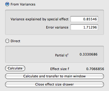 OptionsThis test has no options. |
|
・EXAMPLES 以下の英文内容の日本語の解説 ・数値計算表はこちらです→ [EXCELファイル] ・偏相関係数の数値は、SPSSによるη2とG*Powerのη2とでは違いがあります。 変換式はこちらです→[SPSS η20 vs. G*Power η2] Examples
To illustrate the test of main effects and interaction we assume the specific values for an A × B × C design as illustrated here: 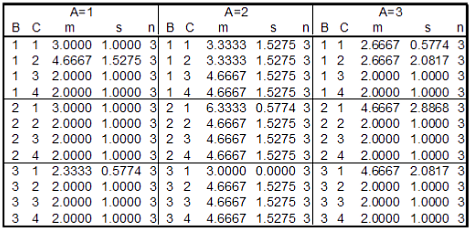 Note, however, that we use this sample data example for didactical purposes only. In G*Power, the input consists of population parameters, not sample statistics. The next table shows the results of a SPSS analysis (GLM univariate) performed on these data. We will show how to reproduce the values in the Observed Power column in the SPSS output with G*Power. 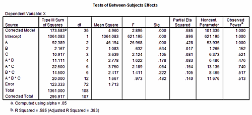 As a first step we calculate the grand mean of the data. Since all groups have the same size (n = 3) this is just the arithmetic mean of all 36 groups means: mg = 3.1382. We then subtract this grand mean from all cells (this step is not essential but makes the calculation and discussion easier). Next, we estimate the common variance σ within each group by calculating the mean variance of all cells, that is, σ2 = 1/36 ∑i s2i = 1.71296. Main effectsIn order to calculate the power for the A, B, and C main effects we need to know the effect size f = σm/σ. We already know σ2 to be 1.71296. We still need to calculate the variance of the means σ2m for each factor. The procedure is analogous for all three main effects. We therefore demonstrate only the calculations necessary for the main effect of factor A.We first calculate the three means for factor A: μi⋆⋆ = {−0.722231, 1.30556, −0.583331}. Due to the fact that we have first subtracted the grand mean from each cell we have ∑i μi⋆⋆ = 0, and we can easily compute the variance of these means as mean square: σ2m = 1/3 ∑i μ2i⋆⋆ = 0.85546. With these values we calculate f = √(σm/σ) = √(0.85546/1.71296) = 0.7066856. The effect size drawer in G*Power can be used to do the last calculation: We choose From Variances and insert 0.85546 in the Variance explained by special effect and 1.71296 in the Error variance field. Pressing the Calculate button gives the above value for f (i.e., 0.7066856) and a partial η2 of 0.3330686. Note that the partial η2 given by G*Power is calculated from f according to the following formula: η2 = f2 /(1 + f2)It is not identical to the SPSS partical η2, which is based on sample estimates. The relation between the two is "SPSS η20" = η2 N/(N + k(η2 − 1)),where N denotes the total sample size, k the total number of groups in the design and η2 the G*Power value. Thus, η20 = 0.33306806 μ 108/(108 + 0.33306806 μ 36 − 36) = 0.42828, which is the value given in the SPSS output. We now use G*Power to calculate the power for α = 0.05 and a total sample size of 3 μ 3 μ 4 μ 3 = 108. We set SelectType of power analysis: Post hoc InputEffect size f : 0.7066856 OutputNoncentrality parameter λ: 53.935690The value of the noncentrality parameter and the power computed by G*Power are identical to the values in the SPSS output. Two-factor interactionsTo calculate the power for two-factor interactions A × B, A × C, and A × B we need to calculate the effect size f corresponding to the values given in the table displayed above. The procedure is analogous for each of the three two-factor interactions. We thus restrict ourselves to the A × B interaction.The values needed to calculate σ2m are the 3 × 3 = 9 residuals δij⋆ . They are given by δij⋆ = μij⋆ − μi⋆⋆ −μ⋆j⋆ = {0.555564, -0.361111, -0.194453, -0.388903, 0.444447, -0.0555444, -0.166661, -0.0833361, 0.249997}. The mean of these values is zero (as a consequence of subtracting the grand mean). Thus, the variance σm is given by 1/9 ∑i,j δ2ij⋆ = 0.102881. This results in an effect size of f = √(0.102881/1.71296) = 0.2450722 or, in terms of the proportion of variance explained, in η2 = 0.0557195. Using the formula given in the previous section on main effects it can be checked that this corresponds to an "SPSS η20" of 0.0813, which is identical to the value given in the SPSS output. We use G*Power to calculate the power for α = 0.05 and a total sample size of 3 × 3 × 4 × 3 = 108. We set: SelectType of power analysis: Post hoc InputEffect size f : 0.2450722 OutputNoncentrality parameter λ: 6.486521 (The notation #A in the comment above means number of levels in factor A). A check reveals that the value of the noncentrality parameter and the power computed by G*Power are identical to the values for (A * B) in the SPSS output. Three-factor interationsTo calculate the effect size of the three-factor interaction corresponding to the values given in table 7 we need the variance of the 36 residuals δijk = μijk − μi⋆⋆ − μ⋆j⋆ − μ⋆⋆k − δij⋆ − δi⋆j − δ⋆jk = {0.333336, 0.777792, -0.555564, -0.555564, -0.416656, -0.305567, 0.361111, 0.361111, 0.0833194, - 0.472225, 0.194453, 0.194453, 0.166669, -0.944475, 0.388903, 0.388903, 0.666653, 0.222242, -0.444447, -0.444447, -0.833322, 0.722233, 0.0555444, 0.0555444, -0.500006, 0.166683, 0.166661, 0.166661, -0.249997, 0.083325, 0.0833361, 0.0833361, 0.750003, -0.250008, - 0.249997, -0.249997}. The mean of these values is zero (as a consequence of subtracting the grand mean). Thus, the variance σm is given by 1/36 ∑i,j,k δ2ijk = 0.185189. This results in an effect size f = √(0.185189/1.71296) = 0.3288016 which is equivalent to η2 = 0.09756294.Using the formula given in the previous section on main effects it can be checked that this corresponds to an "SPSS η2" of 0.140, which is identical to that given in the SPSS output. We use G*Power to calculate the power for α = 0.05 and a total sample size of 3 × 3 × 4 × 3 = 108. We set: Select Type of power analysis: Post hoc InputEffect size f : 0.3288016 OutputNoncentrality parameter λ: 11.675933 (The notation #A in the comment above means number of levels in factor A). Again a check reveals that the value of the noncentrality parameter and the power computed by G*Power are identical to the values for (A * B * C) in the SPSS output. |
Using conventional effect sizesIn the example given in the previous section, we assumed that we know the true values of the mean and variances in all groups. We are, however, rarely in such a privileged position. Instead, we usually only have rough estimates of the expected effect sizes. In these cases we may resort to the conventional effect sizes proposed by Cohen.Assume that we want to calculate the total sample size needed to achieve a power of 0.95 in testing the A × C two-factor interaction at α level 0.05. Assume further that the total design in this scenario is A × B × C with 3 × 2 × 5 factor levels, that is, 30 groups. Theoretical considerations suggest that there should be a small interaction. We thus use the conventional value f = 0.1 defined by Cohen (1969) as small effect. The inputs into and outputs of G*Power for this scenario are: Select
Type of power analysis: A priori InputEffect size f : 0.1 OutputNoncentrality parameter λ: 22.830000 Power for planned comparisonsTo calculate the effect size f = σm/σ for a given comparison C = ∑i=1.. k μi ci we need to know both the standard deviation σ within each group and the standard deviation σm of the effect. The latter is given by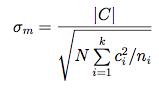 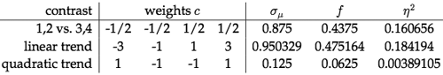 Each contrast has a numerator df = 1. The denominator dfs are N - k, where k is the number of levels (4 in the example). To calculate the power of the linear trend at α = 0.05 we specify: Select Type of power analysis: Post hoc InputEffect size f : 0.475164 OutputNoncentrality parameter λ: 4.515617Inserting the f 's for the other two contrasts yields a power of 0.451898 for the comparison of "1,2 vs. 3,4", and a power of 0.057970 for the test of a quadratic trend. ANOVA: Fixed effects, omnibus, one-way Implementation notesThe distribution under H0 is the central F (df1, N − k) distribution. The numerator df1 is specified in the input and the denominator df is df2 = N − k, where N is the total sample size and k the total number of groups in the design. The distribution under H1 is the noncentral F (df1, N − k, λ) distribution with the same df 's and noncentrality parameter λ = f2 N.ValidationThe results were checked against the values produced by GPower 2.0. Sonntag, 27. 03. 2011
Letzte Änderung: 19.04.2010, 11:49
|